Hello Learners! article: Algorithm Analysis for Novices
If you’re thinking about starting to learn programming or have already started but are struggling to build your logic, feeling overwhelmed by coding, and unsure where to begin, then this page is for you. You’re most welcome!
For beginners, algorithm analysis is a key concept that can help you overcome your fear of Data Structures and Algorithms.
Exactly! Once you start studying algorithm analysis, you’ll become familiar with all the basic concepts frequently used in coding.
In this article, we will cover every important detail related to algorithm analysis.
Introduction
How many cities with more then 250,000 people lie within 500 miles of Noida Delhi?
How many people in my company make over $100,000 per year? Can we connect all of our telephone customers with less than 1,000 miles of cable? To answer questions like these, it is not enough to have the necessary information.
We must organize that information in a way that allows us to find the answers in time to satisfy our needs.
Representing information is fundamental to computer science. The primary purpose of most computer programs is not to perform calculations, but to store and retrieve information – usually as fast as possible.
For this reason, the study of data structures and the algorithms that manipulate them is at the hear of computer science. And that is what this article is about – helping you to understand how to structures information to support efficient processing.
A Philosophy of Data Structures
You might think that with ever more powerful computers, program efficiency is becoming less important. After all, processor speed and memory size still continue to improve. Won’t any efficiency problem we might have today be solved by tomorrow’s hardware?
As we develop more powerful computers, our history so far has always been to use that additional computing power to tackle more complex problems, be it in the from of more sophisticated user interfaces, bigger problem sizes, or new problems previously deemed computationally infeasible.
More complex problems demand more computation, making the need for efficient programs even greater. Worse yet, as tasks become more complex, they become less like our everyday experience.
In the most general sense, a data structure is any data representation and its associated operations. Even an integer or floating point number stored on the computer can be viewed as a simple data structure.
More commonly, people use the term “data structure” to mean an organization or structuring for a collection of data items.
A sorted list of integers stored in an array is an example of such a structuring.
Given sufficient space to store a collection of data items, it is always possible to search for specified items within the collection, print or otherwise process the data items, in any desired order, or modify the value of any particular data item.
Thus, it is possible to perform all necessary operations on any data structure.
However, using the proper data structure can make the difference between a program running in a few seconds and one requiring many days.
When selecting a data structure to solve a problem, you should follow these steps.
- Analyze your problem to determine the basic operations that must be supported.
Examples of basic operations include inserting a data item into the data structure, deleting a data item from the data structure, and finding a specified data item. - Quantify the resources constraints for each operation.
- Select the data structure that best meets these requirements.
This three-step approach to selecting a data structure operationalizes a data-centered view of the design process. The first concern is for the data and the operations to be performed on them, the next concern is the representation for those data, and the final concern is the implementation of that representation.
Resource constraints on certain key operations, such as search, inserting data records, and deleting data records, normally drive the data structure selection process.
Many issues relating to the relative importance of these operations are addressed by the following three questions, which you should ask yourself whenever you must choose a data structure:
- Are all data items inserted into the data structure at the beginning, or are insertions interspersed with other operations?
Static applications (where the data are loaded at the beginning and never change) typically require only simpler data structures to get an efficient implementation then do dynamic applications. - Can data items be deleted? If so, this will probably make the implementation more complicated.
- Are all data items processed in some well-defined order, or is search for specific data items allowed? “Random access” search generally requires more complex data structures.
What is Data Types?
Before getting in to the definition of data types, first understand variables, let us relate them to an old mathematical equation, Many of us would have solved many mathematical equations since childhood. As an example, consider the equations below:
x2 + 2y – 2 = 1
We don’t have to worry about the use of this equation. The important thing that we need to understand is that the equation has names (x and y), which hold values (data).
That means the name (x and y) are placeholders for representing data.
Similarly, in computer science programming we need something for holding data, and variables is the way to do that.
Now come to the point,
In the above-mentioned equation, the variables x and y can take any values such as integral numbers (10, 20), real numbers (0.23, 5.5), or just 0 and 1.
To solve this equation, we need to relate them to the kind of values they can take, and data types is the name used in computer science programming for this purpose.
A data type in a programming langauge is a set of data with predefined values. Examples of data types are: integer, floating point, unit number, character, string, etc.
Computer memory is all filled with zeros and ones. If we have a problem and we want to code it, it’s very difficult to provide the solution in terms of zeros and ones.
To help users, programming langauge, and compilers provide us with data types.
For example, integer takes 2 bytes (actual value depends on compiler), float takes 4 bytes, etc.
This says that in memory we are combining 2 bytes (16 bits) and calling it an integer. Similarly, combining 4 bytes (32 bits) and calling it and float.
A data type reduces the coding effort. At the top level, there are two types of data types:
- System-defined data types (also called Primitive data types)
- User – defined data types.
System-defined data types (Primitive data types)
Data types that are defined by system are called primitive data types. The primitive data types provided by many programming langauge are: int, float, char, double, bool, etc.
The number of bits allocated for each primitive data type depends on the programming languages, the compiler and the operating system. For the same primitive data type, different langauge may use different sizes. Depending on the size of the data types, the total available values (domain) will also change.
For example, “int” may take 2 bytes or 4 bytes. If it takes 2 bytes (16 bits), then the total possible values are -32,768 to +32,767 (-215 to 215-1).
If it takes 4 bytes (32 bits), then the possible values are between -2,147,483,648 and +2,147,483,647. The same is the case with other data types./h
User-defined data types
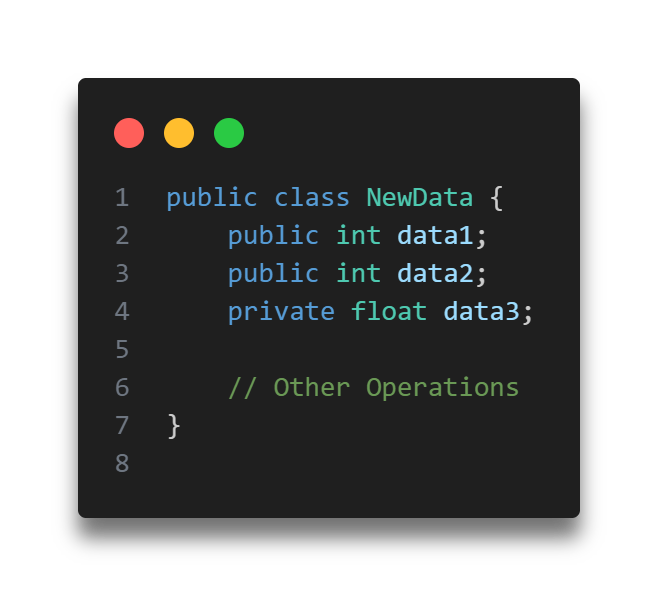
If the system-defined data types are not enough, then most programming languages allow the users to define their own data types, called user – defined data types.
Good examples of user defined data types are: structures in C/C++ and classes in Java.
For example, in the snippet below, we are combining many system-defined data types and calling the user defined data type by the name “newType“.
This gives more flexibility and comfort in dealing with computer memory.
Data Structure
Based on the discussion above, once we have data in variables, we need some mechanism for manipulating that data to solve problems. Data structure is a particular way of storing and organizing data in a computer so that it can be used efficiently.
A data structure is a special format for organizing and storing data. General data structure types include arrays, files, linked list, stacks, queues, trees, graphs and so on.
Depending on the organization of the elements, data structures are classified into two types:
- Linear data structures: Elements are accessed in a sequential order but it is not compulsory to store all elements sequentially (say, Linked Lists). Examples: Linked Lists, Stacks and Queues.
- Non – linear data structures: Elements of this data structure are stored/accessed in a non-linear order. Examples: Tress and graphs.
Abstract Data Types (ADTs)
Before defining abstract data types, let us consider the different view of system-defined data types. We all know that, by default, all primitive data types (int, float, etc.) support basic operations such as addition and subtraction. The system provides the implementations for the primitive data types.
For user-defined data types we also need to define operations. The implementation for these operations can be done when we want to actually use them. That means, in general, user defined data types are defined along with their operations.
To simplify the process of solving problems, we combine the data structures with their operations and we call this Abstract Data Types (ADTs).
An ADT consists of two parts:
- Declaration of data
- Declaration of operations
Commonly used ADTs include: Linked Lists, Stacks, Queues, Priority Queues, Binary Trees, Dictionaries, Disjoint Sets (Union and Find), Hash Tables, Graphs, and many others.
For example, stack uses a LIFO (Last-In-First-Out) mechanism while storing the data in data structures.
The last element inserted into the stack is the first element that gets deleted. Common operations are: creating the stack, push an element onto the stack, pop an element form the stack, finding the current top of the stack, finding the number of elements in the stack, etc.
While defining the ADTs do not worry about the implementation details. They come into the picture only when we want to use them. Different kinds of ADTs are suited to different kinds of applications, and some are highly specialized to specific tasks.
What is an Algorithm?
Let us consider the problem of preparing on omelet. To prepare an omelet, we follow the steps given below:

What we are doing is, for a given problem (preparing an omelet), we are providing a step-by-step procedure for solving it. The formal definition of an algorithm can be stated as:
An algorithm is the step-by-step unambiguous instruction to solve a given problem.
In the traditional study of algorithms, there are two main criteria for judging the merits of algorithms: correctness (does the algorithm give solution to the problem in a finite number of steps?) and efficiency (how much resources ( in terms of memory and time) does it take to execute the).
Note: We do not have to prove each step of the algorithm.
Why the Analysis of Algorithms?
To go from city “A” to city “B”, there can be many ways of accomplishing this: by flight, by bus, by train and also by bicycle. Depending on the availability and convenience, we choose the one the suits us. Similarly, in computer science, multiple algorithms are available for solving the same problem (for example, a sorting problem has many algorithms, like insertion sort, selection sort, quick sort and many more). Algorithm analysis helps us to determine which algorithm is most efficient in terms of time and space consumed.
Goal of the Analysis of Algorithms
The goal of the analysis of algorithms is to compare algorithms (or solutions) mainly in terms of running time but also in terms of other factors (e.g., memory, developer effort, etc.)
What is Running Time Analysis?
It is the process of determining how processing time increases as the size of the problem (input size) increases. Input size is the number of elements in the input, and depending on the problem type, the input may be of different types. The following are the common types of inputs.
- Size of an array
- Polynomial degree
- Number of elements in a matrix
- Number of bits in the binary representation of the input
- Vertices and edges in a graph.
How to Compare Algorithms
To compare algorithms, let us define a few objective mesaures:
Execution times? Not a good measure as execution time are specific to a particular computer.
Number of statements executed? Not a good measure, since the number of statements varies with the programming language as well as the style of the individual programmer.
Ideal solution? Let us assume that we express the running time of a given algorithm as a function of the input size n (i.e., f(n)) and compare these different functions corresponding to running times. This kind of comparison is independent of machine time, programming style, etc.
What is Rate of Growth?
The rate at which the running time increases as a function of input is called rate of growth. Let us assume that you go to a show to buy a car and a bicycle. If your friend sees you there and asks what you are buying, then in general you say buying a car.
This is because the code of the car is high compared to the cost of the bicycle (approximating the cost of the bicycle to the cost of the car).
Total Cost = cost_of_car + cost_of_bicycle
Total Cost ≈ cost_of_car(approximation)
For the above-mentioned example, we can represent the cost of the car and the cost of the bicycle in terms of function, and for a given functions ignore the low order terms that are relatively insignificant (for large value of input size, n).
As an example, in the case below, n4 , 2n2 , 100n and 500 are the individual cost of some function and approximate to n4 since n4 is the highest rate of growth.
n4 + 2n2 + 100n + 500 ≈ n4
Commonly used Rate of Growth
Below is the list of growth rates you will come across in the following.
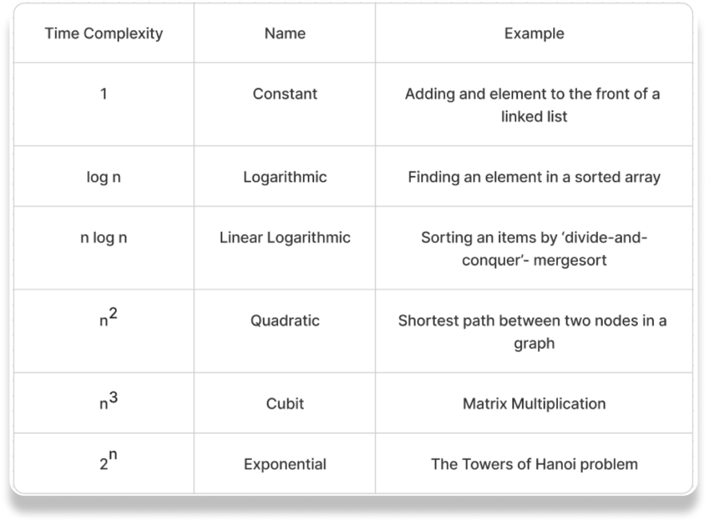
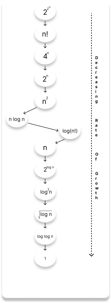
The diagram below shows the relationship between different rates of growth.
Types of Analysis
To analyze the given algorithm, we need to know with which inputs the algorithm takes less time (performing well) and with which inputs the algorithm takes a long time.
We have already seen that an algorithm can be represented in the form of an expression. That means we represent the algorithm with multiple expressions: one for the case where it takes less time and another for the case where it takes more time.
In general, the first case is called the best case and the second case is called the worst case for the algorithm. To analyze an algorithm we need some kind of syntax, and that forms the base for asymptotic analysis/notation.
There are three types of analysis:
- Worst case
- Defines the input for which the algorithm takes a long time (slowest time to complete).
- Base case
- Defines the input for which the algorithm takes the least time (fastest time to complete).
- Input is the one for which the algorithm runs the fastest.
- Average case
- Provides a prediction about the running time of the algorithm.
- Run the algorithm many times, using many different inputs that come from some distribution that generates these inputs, compute the total running time (by adding the individual times), and divide by the number of trials.
- Assumes that the input is random.
Lower Bound <= Average Time <= Upper Bound
For a given algorithm, we can represent the best, worst and average cases in the form of expressions.
As an example, let f(n) be the function, which represents the given algorithm.
f(n) = n2 + 500, for worst case
f(n) = n + 100n + 500, for best case
Similarly for the average case. The expression defines the inputs with which the algorithm takes the average running time (or memory).
Asymptotic Notation
Having the expressions for the best, average and worst case, for all three cases we need to identify the upper and lower bounds. To represent these upper and lower bounds, we need some kind of syntax, and that is the subject of the following discussion. Let us assume that the given algorithm is represented in the form of function f(n).
Big-O Notation
This notation gives the tight upper bound of the given function.
Generally, it is represented as f(n) = O(g(n)). That means, at larger values, of n, the upper bound of f(n) is g(n).
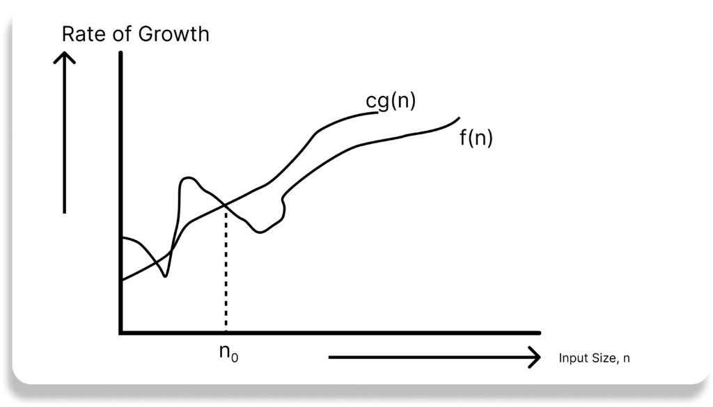
Big O notation (with a capital letter O, not a zero), also called Landau’s symbol, is a symbolism used in complexity theory, computer science, and mathematics to describe the asymptotic behavior of functions.
Landau’s symbol comes from the name of the German number theoretician Edmund Landau who invented the notation. The letter O is used because the rate of growth of a function is also called its order.
Big O notation tells you how much slower a piece of a program gets as the input gets larger. For example:
- Returning the first element of an array takes a constant amount of time. If you double the length of an array, it still takes the same amount of time. That code does not scale with input size.
- Summing all the elements of an array takes a linear amount of time with regard to the length of the array. Double the length, the code takes roughly twice as long. Make the array a hundred times longer, code takes a hundred times as long.
- Searching for an element in a sorted array? If you’re using a binary search, every time the array length is doubled you need to add one extra comparison. Performance does get worse as the array length increases, but less than linearly.
The notation of Big O notation is just concise shorthand for describing the above patterns. O(1) for constant time, O(n) for linear time (where n is the length of the array), O (log n) for logarithmic time, etc.
The focus of Big O notation is on looking at the biggest trend of an algorithm. We don’t care whether an algorithm takes 200 steps or 201 steps, we just care about how it scales as input size changes.
Therefore, we only look at the slowest part of an algorithm. O(n + 1) simplifies to O(n), because as the array size gets millions of times longer the O(1) is quite insignificant.
Here is a list of classes of functions that are commonly encountered when analyzing algorithms.
| Notation | Name |
| O(1) | constant |
| O(log(n)) | logarithmic |
| O((log(n))c) | polylogarithmic |
| O(n) | linear |
| O(n2) | quadratic |
| O(nc) | polynomial |
| O(cn) | exponential |
Omega-Ω Notation
Similar to the O discussion, this notation gives the tighter lower bound of the given algorithm and we represent it as f(n) = Ω(g(n)). That means, at larger values of n, the tighter lower bound of f(n) if g(n). For example, if f(n) = 100n2 + 10n + 50, g(n) is Ω(n2).
The Ω notation can be defined as Ω(g(n)) = { f(n): there exist positive constants c and n0 such that 0 <= cg(n) <= f(n) for all n >= n0 }.
g(n) is an asymptotic tight lower bound for f(n). Our objective is give the largest rate of growth g(n) which is less than or equal to the given algorithm’s rate of growth f(n).
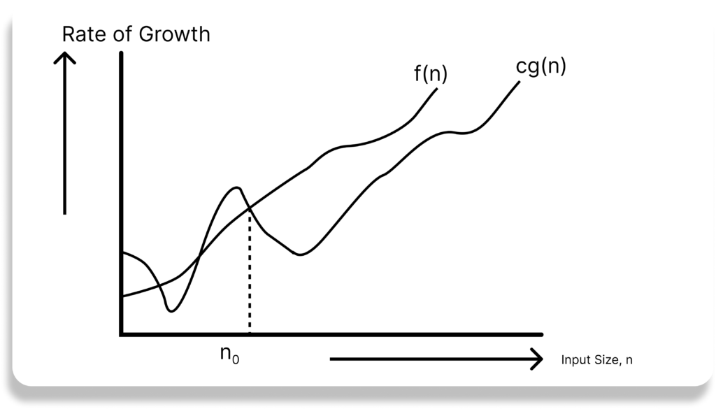
Imagine you have an algorithm that sorts a list of numbers. In the best-case scenario, the lit might already be sorted. Omega notation helps us understand the least amount of time it would take the algorithm to check and finish the task.
For example: If an algorithm’s time complexity is Ω(n)m it means that in the best case, the algorithm will take at least linear time (proportional to the size of the input, n) to finish. No matter what, it won’t run faster than that.
So, in short: Omega (Ω) notation tells us how fast an algorithm can run in the best situation.
Theta-Θ Notation
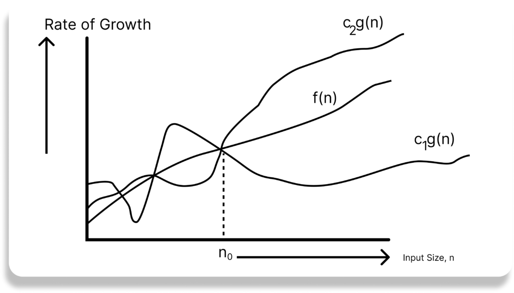
This notation decides whether the upper and lower bounds of a given function (algorithm) are the same. The average running time of an algorithm is always between the lower bound and the upper bound. If the upper bound (O) and lower bound(Ω) give the same result, then the Θ notation will also have the same rate of growth.
As an example, let us assume that f(n) = 10n + n is the expression. then, its right upper bound g(n) is O(n). The rate of growth in the best case is g(n) = O(n).
In this case, the rates of growth in the best case and worst case are the same. As a result, the average case will also be the same. For a given function (algorithm), if the rates of growth (bounds) for O and Ω are not the same, then the rate of growth for the Θ case may not be the same.
Now consider the definition of Θ notation. It is defined as Θ(g(n)) = { f(n): there exist positive constants c1, c2 name n0 such that 0 <= c1g(n) <= f(n) <= c2g(n) for all n >= n0 }. g(n) is an asymptotic tight bound for f(n). Θ(g(n)) is the set of functions with the same order of growth as g(n).
Why is it called Asymptotic Analysis?
From the discussion above (for all three notations: worst case, best case, and average case), we can easily understand that, in every case for a given function f(n) we are trying to find anther function g(n) which approximates f(n) at higher values of n.
That means g(n) is also a curve which approximates f(n) at higher values of n.
In mathematics we call such a curve an asymptotic curve. In other terms, g(n) is the asymptotic curve for f(n). For this reason, we call algorithm analysis asymptotic analysis.
Guidelines for Asymptotic Analysis
There are some general rules to help us determine the running time of an algorithm.
- Loops: The running time of a loop is, at most, the running time of the statements inside the loop (including tests) multiplied by the number of iterations.
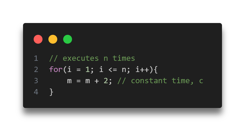
Total time = a constant c × n = c n = O(n).
- Nested Loops: Analyze from the inside out. Total running time is the product of the sizes of all the loops.
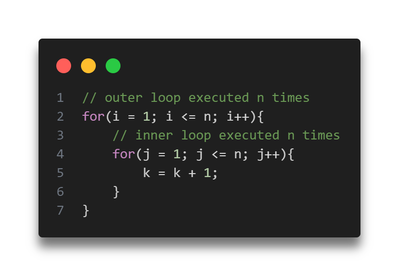
Total time = c × n × n = cn2 = O(n2).
- Consecutive Statements: Add the time complexities of each statement.
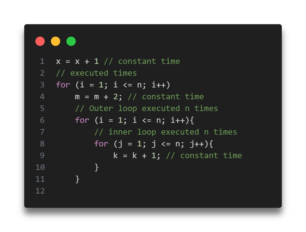
Total time = c0 + c1n + c2n2 = O(n2).
- If-then-else statement: Worst-case running time: the test, plus either the then part or the else part (whichever is the larger).
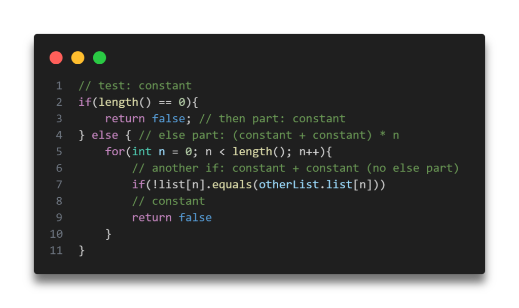
Total time = c0 + c1 + (c2 + c3) * n = O(n).
- Logarithmic complexity: An algorithm is O(logn) if it takes a constant time to cut the problem size by a fraction (usually by 1/2). As an example let us consider the following program:
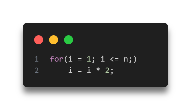
If we observe carefully, the value of i doubling every time. Initially i = 1, in next step i = 2, and in subsequent steps i = 4, 8 and so on. Let us assume that the loop is executing some k times. At kth step 2k = n, and at (k + 1)th step we come out of the loop. Taking logarithm on both sides, gives
log(2k) = logn
klog2 = logn
k = logn // if we assume base 2
Total time = O(logn).
Thank you for taking the time to read! Feel free to explore more of our content or leave a comment below.

Leave a Reply